
GRAVITON / RESEARCH NOTE 02
How much depends
on when we look?
We put an earlier quantum-model result through 180 settings and four observation windows. The wider test shows where the conclusion holds—and where it reverses.
BY GRAVITON ·
Explore the resultsComputational research note · Finite quantum model · No experimental data · Not peer reviewed
01 / WHAT WE FOUND
The earlier result holds.
Its generalization does not.
In our earlier calculation, adding one four-operator interaction reduced the mean absolute autocorrelation during t = 12–24, at each of three positive coupling strengths. Matching the models’ RMS energy removed one simple explanation: an overall change of energy scale.
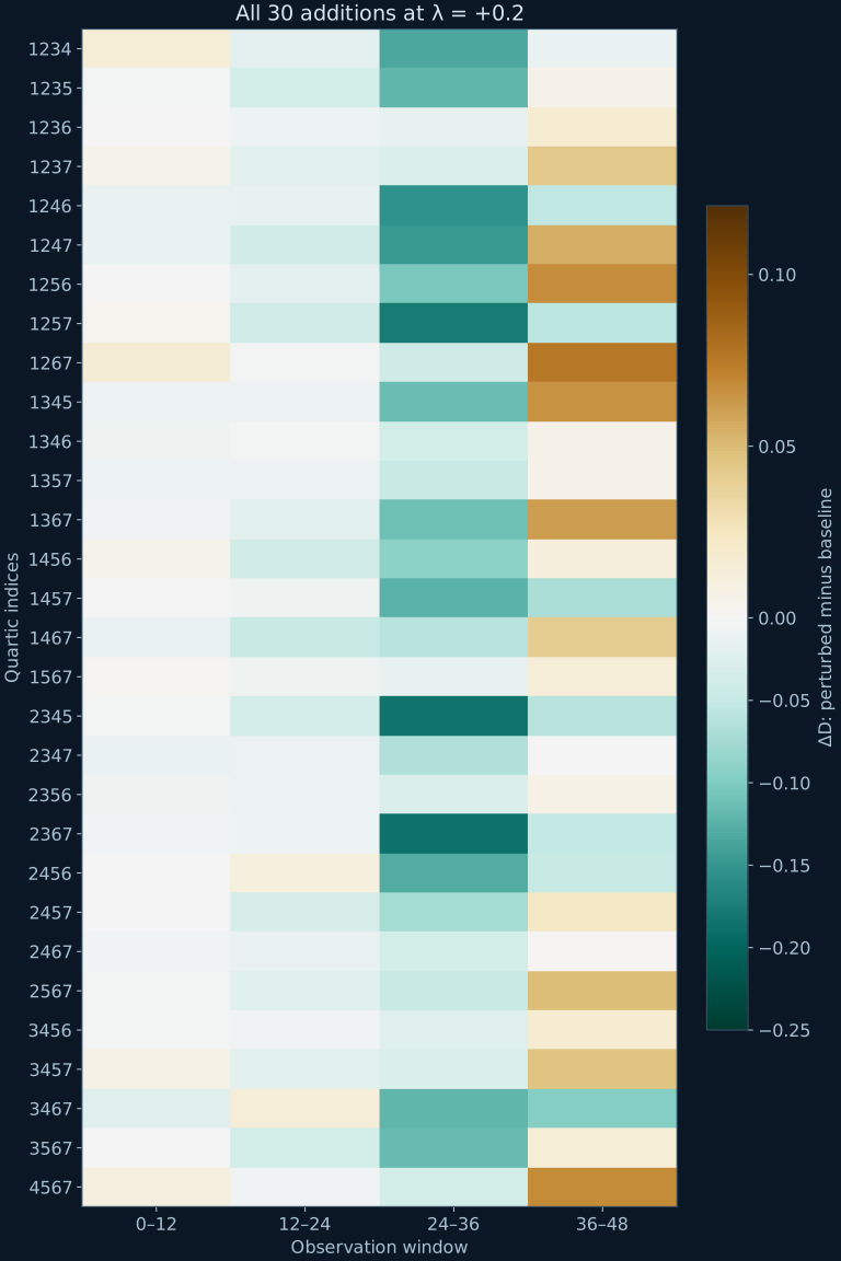
That was a result about a chosen interaction and interval. Here we keep the energy-matching rule and observable, but examine every four-operator addition drawn from the seven active operators that is absent from the baseline. This gives 30 additions, six signed coupling values, and four windows: 720 comparisons across 180 Hamiltonians.
Counts use the declared Δt = 0.1 grid. They describe a finite enumeration, not independent replications or probabilities. With finer grids, the last count becomes 132.
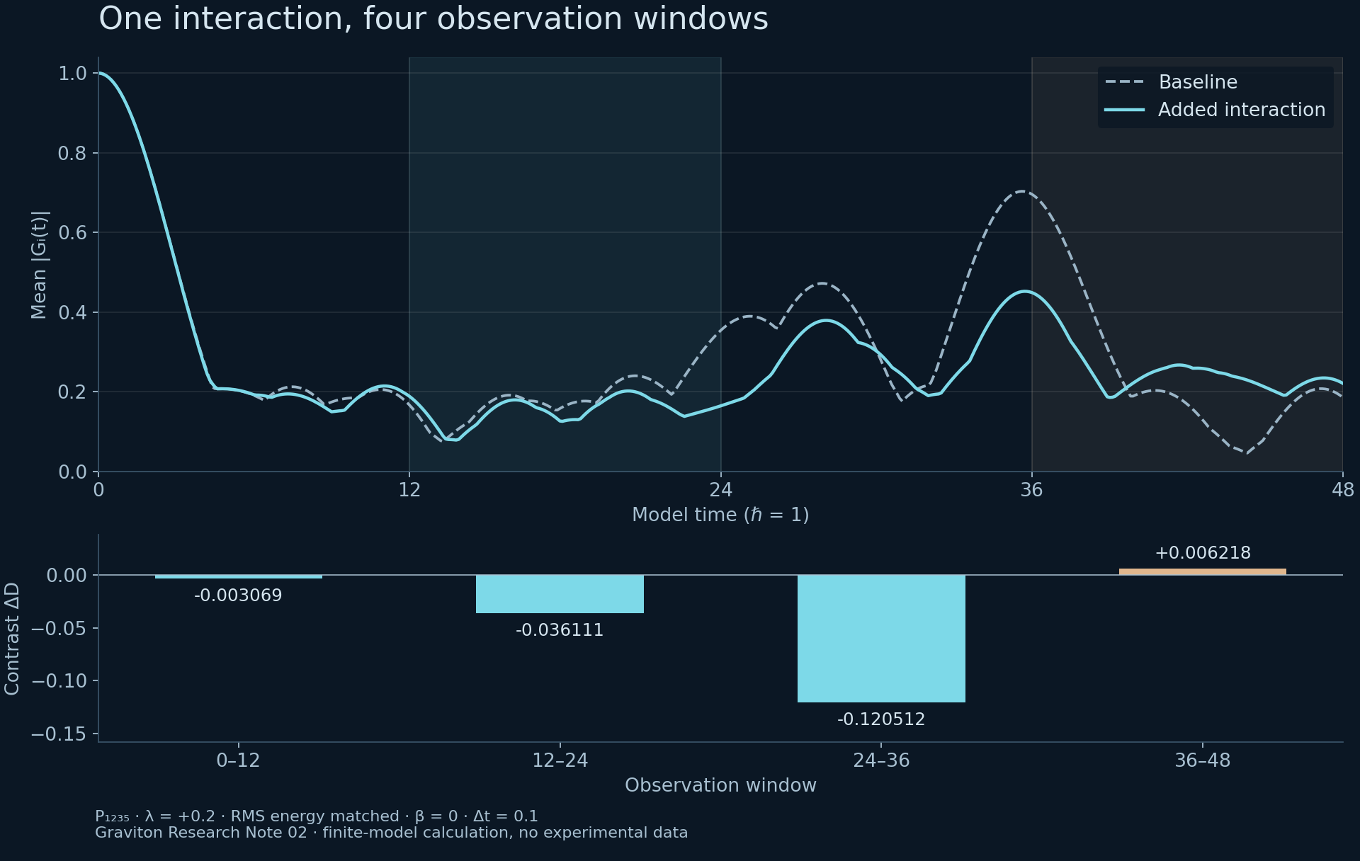
The original addition, ψ₁ψ₂ψ₃ψ₅ at λ = 0.2, provides a particularly clear example. Its contrast is −0.036111 in t = 12–24 and +0.006218 in t = 36–48. Both signs survive the two finer grids. The claim that this addition always reduces the diagnostic therefore fails even before we consider the other interactions.
| Window | Lower average | Higher average |
|---|---|---|
| 0–12 | 116 | 64 |
| 12–24 | 155 | 25 |
| 24–36 | 176 | 4 |
| 36–48 | 96 | 84 |
Two additions, ψ₁ψ₂ψ₆ψ₇ and ψ₄ψ₅ψ₆ψ₇, commute with the baseline Hamiltonian and remain in the enumeration as controls. The remaining 28 do not. Positive contrasts also occur among those noncommuting cases, in every window. The failure is therefore not confined to the commuting controls.
02 / THE COMPLETE COMPARISON
Choose an interaction.
Move the window.
The plot shows the average of the absolute autocorrelations of all seven active operators. The highlighted interval is the one being compared. Every option comes from the downloadable calculation.
Loading the verified calculation. The static figure and results below are available without JavaScript.
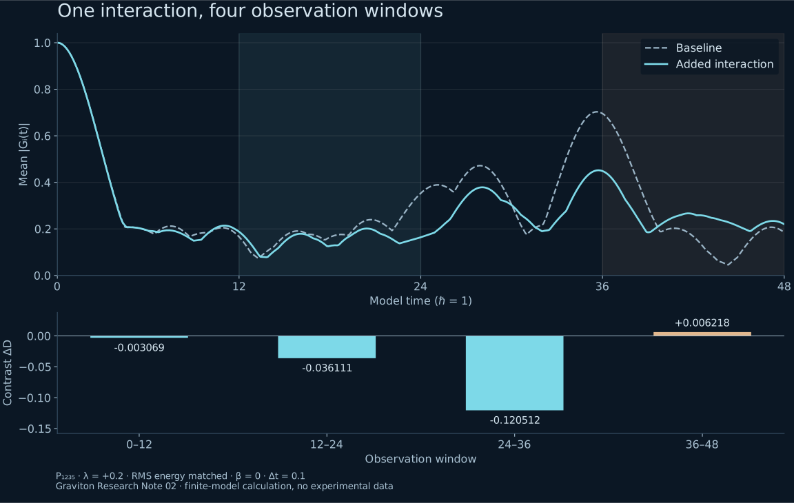
For the reference interaction at λ = 0.2, t = 12–24 gives a lower average. Select t = 36–48 to inspect the reversal.
Inspect all 30 interactions at the selected coupling
Each cell is ΔD for one observation window. Negative means a lower average; positive means a higher one. Select a row to inspect its trace. An asterisk marks a sign that changes between the primary and finest grid. Values near zero deserve particular care.
| Interaction | 0–12 | 12–24 | 24–36 | 36–48 |
|---|
A SHORT CONCEPT GUIDE
What are we comparing?
- Hamiltonian
- The matrix that specifies the system’s energy and generates its time evolution. Here it acts on a 16-dimensional space.
- Majorana operator
- A Hermitian fermionic operator obeying the anticommutation rule below. These matrices are a mathematical representation; this calculation does not create or detect a particle.
- Quartic interaction
- A product of four distinct Majorana operators. Its coefficient λ sets the strength and sign of the added interaction.
- Autocorrelation
- The trace-based overlap between an operator and its later version. The normalized value starts at one. We average its absolute value, so opposite signs do not cancel.
- Commuting
- Two operators commute when their order in a product makes no difference. Adding a noncommuting term changes the dynamics, but does not by itself prove thermalization.
- RMS energy
- The root-mean-square spread of Hamiltonian eigenvalues around their mean. Matching it fixes one overall energy scale; it does not match the full spectrum.
- Observation window
- The interval over which the diagnostic is averaged. A finite system can revisit earlier patterns, so different windows need not agree.
03 / THE SPECIFIED MODEL
One definition,
used throughout.
We use the five-term historical Hamiltonian printed in Kobrin, Schuster and Yao’s 2023 comment. The original experiment and the authors’ response provide the context for the model; our calculation is a separate infinite-temperature diagnostic, not a reproduction of their teleportation protocol. [1–3]
Write Pabcd = ψaψbψcψd, with increasing indices. The baseline is
For each selected P and λ, form A = H₀ + λP, subtract its trace, and rescale:
à = A − Tr(A)I₁₆/16 and r(A) = √[Tr(ò)/16]. All 180 matched models have the same centered RMS energy as H₀. Their spectral shapes and conserved quantities can still differ.
Each primary window contains 121 samples, including both endpoints. The average is a discrete statistic, not a continuous-time integral. Operator ψ₈ commutes with every Hamiltonian in this family and has G₈(t) = 1; it is checked but excluded from D.
Matrix construction and calculation method
On four qubits, ψ₂ⱼ₋₁ = Z⊗(j−1) ⊗ X ⊗ I⊗(4−j) / √2, for j = 1,…,4; replacing X with Y gives ψ₂ⱼ. The notation Z⊗n means n tensor factors of Z. The first qubit is the leftmost factor. This representation fixes all signs and normalizations.
Diagonalizing H = V diag(E)V† gives Gᵢ(t) = (2/16) Σₐᵦ |(V†ψᵢV)ₐᵦ|² cos[(Eₐ − Eᵦ)t]. The main sweep uses this spectral formula. A separate matrix-exponential implementation, using a Taylor series with scaling and squaring, checks every Hamiltonian at t = 0, 6, 12, 18, 24, 36 and 48.
The seven-operator Hamiltonian is embedded in a 16-dimensional representation with an eighth spectator. No physical duration in seconds, laboratory material, or gravitational dual is assigned to this calculation.
04 / WHAT WAS CHECKED
Small numerical errors.
Real sensitivity to the question.
The two evolution methods agree to within 1.5 × 10⁻¹⁴ on the stated check points. Normalization, Hermiticity, spectator conservation and RMS matching pass the declared 10⁻¹⁰ tolerance. The three earlier reference contrasts are recovered to within 5.3 × 10⁻¹⁶.
We also repeat every window average at Δt = 0.05 and 0.025. Six of the 720 contrasts change sign between the primary and finest grids: P₁₃₅₇ at λ = ±0.3 in windows 24–36 and 36–48, and P₂₃₅₆ at λ = ±0.3 in window 36–48. The maximum contrast shift is 0.001985, rounded upward. The two finer grids agree on all contrast signs.
We retain the original grid and report its sensitivity. The finite-grid statistic changes when its sampling rule changes; these differences are not solver failures or statistical error bars. They are also not a rigorous bound on the continuous-time average. The broad failure of an always-negative contrast remains on every grid.
The protocol was saved before this sweep ran. It was not externally preregistered: the earlier reference result was already known. All 30 additions, six couplings and four windows are retained. The models are related, some outputs coincide, and none of these counts should be read as independent experimental confirmations.
The inference is deliberately narrow. This diagnostic depends on the interaction and the observation window. The calculation does not measure teleportation, operator-size winding, entanglement growth, an out-of-time-order correlator, or a thermalization rate. It therefore cannot settle the wider dispute about gravitational interpretations of the original experiment.
05 / THE NEXT RESEARCH STEP
Choose the physical question
before choosing the score.
Our next task in this branch is to connect a measured quantity to a specific physical claim. For equilibration, that means specifying the subsystem and initial-state family, accounting for conserved components, and comparing local observables over windows chosen before the results are seen. A recent preprint develops finite-window bounds for a different, stationary-subtracted mean-square diagnostic; its assumptions and observable would need a separate implementation. We do not apply those bounds to D. [4]
For a gravitational interpretation, agreement of a single autocorrelation average is insufficient. A stronger study would compare several independently defined observables, include suitable nongravitational alternatives, and investigate how the distinction behaves as system size grows. The present note supplies a reproducible reason to demand that broader comparison.
METHODS / SOURCES / REPRODUCIBILITY
Read it. Run it.
Check it.
The Hamiltonian comes from the cited literature. Graviton’s contribution here is the stated finite sweep, its checks, and the interpretation of its limits. We make no priority claim for the diagnostic or the general observation that finite-window conclusions can vary.
python3 -m pip install numpy
python3 verify-robustness.py
Keep the script and protocol.json in the same folder. Requires Python 3.10+ and NumPy. The current run used NumPy 2.3.5. The JSON records source hashes, numerical tolerances and all results. When the earlier site dataset is present, the script also checks the historical reference values.
- Jafferis, D. et al. (2022). Traversable wormhole dynamics on a quantum processor. Nature 612, 51–55. Context for the experimental program.
- Kobrin, B., Schuster, T. & Yao, N. Y. (2023). Comment on “Traversable wormhole dynamics on a quantum processor”. arXiv:2302.07897. Source of the five-term Hamiltonian and its normalization.
- Jafferis, D. et al. (2023). Response to the comment. arXiv:2303.15423. Authors’ interpretation and the reference quartic perturbation.
- Ćwikliński, P. (2026). Finite-time quantum equilibration from local correlations. Preprint, version 2, 21 October 2026. A separate framework for future study, not a theorem invoked by this calculation.